See who opens your spreadsheets
Share as a tracked Sizle link. Get instant open alerts & engagement insights.
Trusted by 30,000+ users. No credit card needed.
If you have ever wanted to categorize numeric information collectively, you’ve come to the right place! SUMIF is a useful function that you’ll probably end up using all the time after this.
When you break it down, SUMIF in Google Sheets is exactly what the name implies: The sum of data if it matches your specified guidelines.
If SUMIF sounds somewhat familiar to you, you might be thinking of its less meticulous little brother, SUM. You can find SUM throughout all standard computer courses that teach the basics of programs like Excel and Google Sheets.
The SUMIF function in Google Sheets takes SUM a little further. It allows you to find the basic total (SUM) and a whole lot more.
How to Use SUMIF in Google Sheets
Using SUMIF in Google Sheets isn’t super complicated. In fact, if you’ve used it in Excel, you’ll be reasonably familiar with the premise. The formula used looks a little intimidating, but it becomes easy once you know what all the pieces are for.
Key Formula:
“SUMIF(range, criterion,[sum_range])”
At first glance, these terms may seem complex. However, they are pretty straightforward after some practice. Let’s explore each component.
- SUMIF – The function you’re asking the cell you’re working in to prepare to complete.
- Range – the area of the sheet you’d like to add together.
- Criterion – This is the condition you need to have met, whether that’s an amount or some sort of wording
- Sum_Range – The specific cells you’d like the sheet to add together
Without seeing it in action, it can be a bit confusing. Here’s a real-world example to help bring this formula to life.
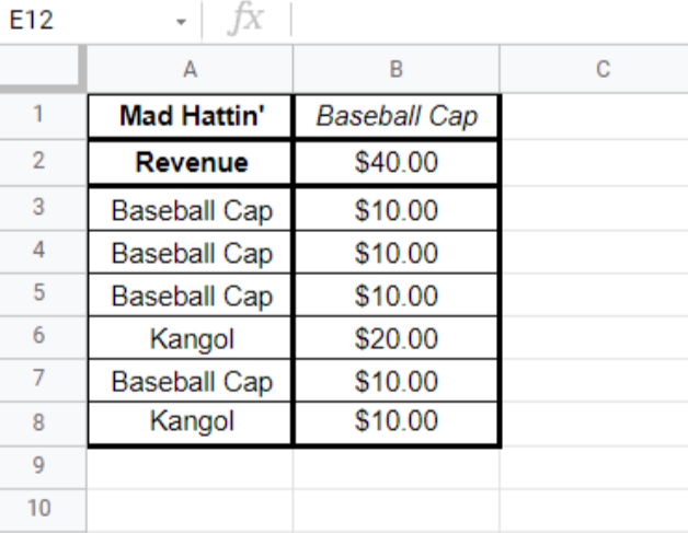
Let’s say you own a store. When reviewing your sales numbers, you needed to know exactly how much you made selling baseball caps. In this case, a SUMIF formula can be quite handy. You might make something like this:

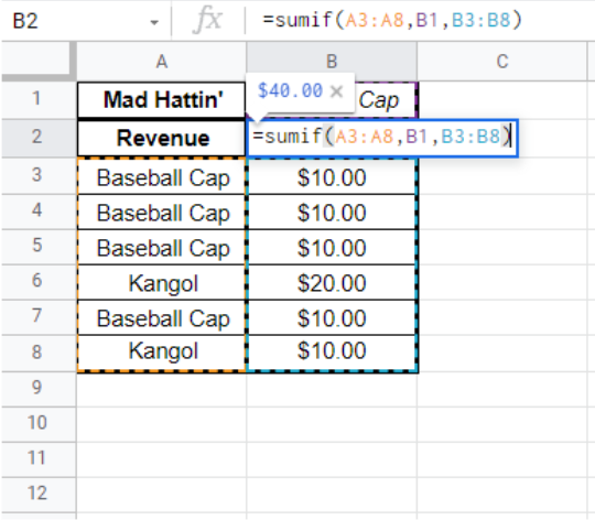
Now, to find out how much you made on baseball caps, you’d enter ‘baseball caps’ in cell B1 and follow with your formula in B2: “=SUMIF(range, criterion,[sum_range])”
- Range (Hats): A3:A8
- Criterion (Baseball Caps): B1
- Sum_Range: B3:B8
Your formula should look like the following: “=SUMIF(A3:A8, B1, B3:B8)”
If you’re following along and are unsure of your cells, you can always use the Find and Replace tool to search for the word you’re looking for in all the cells it exists in.

If you hit enter, and your screen comes back with “$40.00”, you’ve succeeded! If not, you will get an error message, and that is okay. Double click on your cell, and double-check the formula. It was created not to fail you.
Google Sheets SUMIF Multiple Criteria
Using a similar function to SUMIF, multiple criteria in google sheets can only happen when adding an extra ‘S:’ SUMIFS. SUMIFS allows you to include various pieces of data into your formula to get the amount you need in seconds.
The SUMIFS formula is composed of several pieces of criteria. The overarching shell of this magical time-saving tool is:
=SUMIFS(sum_range, criteria_range1, criteria1, [criteria_range2, criteria2], …)
Let’s take a look at what we have going on in there.
We’ll use an imaginary A5:A10-D5:D10.
- =SUMIFS(A5:A10, – This is the sum_range, which is the area that you want to be added/summed by the end of your input.
- B5:B10 – This next one is your first criteria range. The purpose of this formula is to locate the data that corresponds to the first range given.
- “=baseball*”, – This is a Wildcard Character attached to your specified criteria. It identifies the command even further. For example, you can use this modifier if you need to only get the sums for the products that have to do with baseball.
- C5:C10, – Here is the second criteria range. You’ll be able to specify where else you need to pull data from.
- “caps”) – Finally, we have the second criteria. Let’s suppose you’re trying to find how well baseball caps sold that week. Then you should specify ‘caps’ so the formula can pull only those item sales.
In the end, your formula can break down (based on the above example) how many baseball caps you sold, rather than the total number of general cap sales or sales related to all baseball-related merchandise.
SUMIF with Wildcard Characters
Wildcard characters are characters that you do not usually find in a more base level of code. For example, an asterisk [[ * ]] forces a match one or more characters, a question mark will match any single character, while a tilde [[ ~ ]] forces the literal * or ? characters to show themselves.
An example of a SUMIF formula that has wildcard characters would be
“=SUMIF(A3:A8,”*baseball*”,B3:B8)”
This formula, based on the above image, broken down becomes:
- Range: A3:A8 – the products
- Criteria: “*baseball*” – the item that you want to specify
- Sum_Range: B3:B8 – the actual range that to be added/summed by the system
SUMIF Formulas for Dates
Luckily, there is no such thing as a case-sensitive SUMIF formula. That makes finding the formulaic descriptor for dates even simpler.
Here’s an example formula you might use with any cell. In this case, we’ve used imaginary columns C and D.
=SUMIF(C5:C10, date(year,month,day), D5:D10)
Let’s break it down again:
- Range: Cells C5:D10, the dates
- Criteria: date(year,month,day), – your condition, the date you want the formula to pick out
- Sum_Range: Cells D5:D10 – the actual range you’re trying to add together.
As you can see, the formula stays the same. When you want to add something else, you can quickly add these fancy extra modifiers.
Although that was a lot to cover, you don’t have to remember it all right now. That’s why we made a cheat sheet like this one.
SUMIF Function on Google Sheets
Overall, the SUMIF formula is a great way to minimize the time-consuming task of creating spreadsheets with a lot of repetitive information. Being able to sort out the numeric values of specified ranges takes the guesswork out of compiling data. Read on for more Google Sheets and Excel tutorials, tips and tricks!
Close faster. Be deal-ready.
Visibility builds trust. Trust closes deals. Sizle helps you see every step from share to signature.
Free 7-day trial. No card required. Cancel anytime.
Trusted by 30,000+ professionals across 175+ countries
